DL-Model Inference Pipeline#
In this example the construction of an end-to-end DICOM-based auto-segmentation solution using the famous U-Net is demonstrated. The given solution delineates the skull of the patient based on a T1-weighted post-contrast and a T2-weighted image. For this example the provided example data and a given PyTorch-based DL-model is used that both can be found in the example data GitHub repository.
Because PyRaDiSe is DL-framework agnostic to allow for maximum flexibility, PyTorch must be installed to execute this example.
Preparation#
Before getting started with constructing the auto-segmentation solution one needs to import the following packages and modules.
[1]:
from typing import (
    Any,
    Dict,
    Optional)

import torch
import torch.nn as nn
import numpy as np

import pyradise.data as ps_data
import pyradise.fileio as ps_io
import pyradise.process as ps_proc

from network import UNet
InferenceFilter Implementation#
In the following section, the implementation of a PyTorch-based inference filter is demonstrated. This implementation may be used as a starting point for more sophisticated inference filters. Implementation details are mentioned in the code below.
[3]:
class ExampleInferenceFilter(ps_proc.InferenceFilter):
    """An example implementation of an InferenceFilter for
    slice-wise segmentation with a PyTorch-based U-Net."""

    def __init__(self) -> None:
        super().__init__()

        # Define the device on which the model should be run
        self.device = torch.device('cuda' if torch.cuda.is_available() else 'cpu')

        # Define a class attribute for the model
        self.model: Optional[nn.Module] = None

    def _prepare_model(self,
                       model: nn.Module,
                       model_path: str
                       ) -> nn.Module:
        """Implementation using the PyTorch framework."""

        # Load model parameters
        model.load_state_dict(torch.load(model_path, map_location=self.device))

        # Assign the model to the class
        self.model = model.to(self.device)

        # Set model to evaluation mode
        self.model.eval()

        return model

    def _infer_on_batch(self,
                        batch: Dict[str, Any],
                        params: ps_proc.InferenceFilterParams
                        ) -> Dict[str, Any]:
        """Implementation using the PyTorch framework."""

        # Stack and adjust the numpy array such that it fits the
        # [batch, channel / images, height, width, (depth)] format
        # Note: The following statement works for slice-wise and patch-wise processing
        if (loop_axis := params.indexing_strategy.loop_axis) is None:
            adjusted_input = np.stack(batch['data'], axis=0)
        else:
            adjusted_input = np.stack(batch['data'], axis=0).squeeze(loop_axis + 2)

        # Generate a tensor from the numpy array
        input_tensor = torch.from_numpy(adjusted_input)

        # Move the batch to the same device as the model
        input_tensor = input_tensor.to(self.device, dtype=torch.float32)

        # Apply the model to the batch
        with torch.no_grad():
            output_tensor = self.model(input_tensor)

        # Retrieve the predicted classes from the output
        final_activation_fn = nn.Sigmoid()
        output_tensor = (final_activation_fn(output_tensor) > 0.5).bool()

        # Convert the output to a numpy array
        # Note: The output shape must be [batch, height, width, (depth)]
        output_array = output_tensor.cpu().numpy()

        # Construct a list of output arrays such that it fits the index expressions
        batch_output_list = [output_array[i, ...] for i in range(output_array.shape[0])]

        # Combine the output arrays into a dictionary
        output = {'data': batch_output_list,
                  'index_expr': batch['index_expr']}

        return output
Filter Pipeline Construction#
In this section, the construction of the processing pipeline is shown using the inference filter implemented before.
This demonstrated processing pipeline is simple and does not include registration to a reference image that would modify the spatial properties of the input images. Thus, the playback of the transform tapes recoding the changes of the spatial properties is not required. However, in DL practice registration to a reference image is often used and a playback of the transform tapes is essential to generate correctly aligned segmentations. For those cases we recommend to add a PlaybackTransformTapeFilter to the pipeline.
[4]:
def get_pipeline(model_path: str) -> ps_proc.FilterPipeline:
    # Construct a pipeline the processing
    pipeline = ps_proc.FilterPipeline()

    # Construct and ddd the preprocessing filters to the pipeline
    output_size = (256, 256, 256)
    output_spacing = (1.0, 1.0, 1.0)
    reference_modality = 'T1'
    resample_filter_params = ps_proc.ResampleFilterParams(output_size,
                                                          output_spacing,
                                                          reference_modality=reference_modality,
                                                          centering_method='reference')
    resample_filter = ps_proc.ResampleFilter()
    pipeline.add_filter(resample_filter, resample_filter_params)

    norm_filter_params = ps_proc.ZScoreNormFilterParams()
    norm_filter = ps_proc.ZScoreNormFilter()
    pipeline.add_filter(norm_filter, norm_filter_params)

    # Construct and add the inference filter
    modalities_to_use = ('T1', 'T2')
    inf_params = ps_proc.InferenceFilterParams(model=UNet(num_channels=2, num_classes=1),
                                               model_path=model_path,
                                               modalities=modalities_to_use,
                                               reference_modality=reference_modality,
                                               output_organs=(ps_data.Organ('Skull'),),
                                               output_annotator=ps_data.Annotator('AutoSegmentation'),
                                               organ_indices=(1,),
                                               batch_size=8,
                                               indexing_strategy=ps_proc.SliceIndexingStrategy(0))

    inf_filter = ExampleInferenceFilter()
    pipeline.add_filter(inf_filter, inf_params)

    # Add postprocessing filters
    cc_filter_params = ps_proc.SingleConnectedComponentFilterParams()
    cc_filter = ps_proc.SingleConnectedComponentFilter()
    pipeline.add_filter(cc_filter, cc_filter_params)

    # Because the spatial properties of the subject images are
    # changed with respect to the reference T1 image a playback
    # of the TransformTape is not required. If the spatial properties
    # of the reference image would have been changed the playback can
    # be achieved using the PlaybackTransformTapeFilter.
    #
    # playback_params = PlaybackTransformTapeFilterParams()
    # playback_filter = PlaybackTransformTapeFilter()
    # pipeline.add_filter(playback_filter, playback_params)

    return pipeline
Auto-segmentation Pipeline Construction#
The following section demonstrates the construction of the inference procedure that can be split into the following tasks:
Import DICOM images
Generate and run the filter pipeline
Convert segmentation masks to DICOM-RTSS
Serialize DICOM-RTSS and copy the original DICOM images
[5]:
def infer(input_dir_path: str,
          output_dir_path: str,
          model_path: str
          ) -> None:
    # Crawl the data in the input directory
    crawler = ps_io.SubjectDicomCrawler(input_dir_path)
    series_info = crawler.execute()

    # Select the required modalities
    used_modalities = ('T1', 'T2')
    modality_selector = ps_io.ModalityInfoSelector(used_modalities)
    series_info = modality_selector.execute(series_info)

    # Exclude the existing DICOM-RTSS files
    no_rtss_selector = ps_io.NoRTSSInfoSelector()
    series_info = no_rtss_selector.execute(series_info)

    # Construct the loader and load the subject
    loader = ps_io.SubjectLoader()
    subject = loader.load(series_info)

    # Construct the pipeline and execute it
    pipeline = get_pipeline(model_path)
    subject = pipeline.execute(subject)

    # Define the customizable metadata for the DICOM-RTSS
    # Note: Check the value formatting at:
    # https://dicom.nema.org/dicom/2013/output/chtml/part05/sect_6.2.html
    meta_data = ps_io.RTSSMetaData(patient_name='Jack Demo',
                                   patient_id=subject.get_name(),
                                   patient_birth_date='19700101',
                                   patient_sex='F',
                                   patient_weight='80',
                                   patient_size='180',
                                   series_description='Demo Series Description',
                                   series_number='10',
                                   operators_name='Auto-Segmentation Alg.')

    # Convert the segmentations to a DICOM-RTSS
    reference_modality = 'T1'
    conv_conf = ps_io.RTSSConverter3DConfiguration(decimate_reduction=0.5)
    converter = ps_io.SubjectToRTSSConverter(subject,
                                             series_info,
                                             reference_modality,
                                             conv_conf,
                                             meta_data)
    rtss_dataset = converter.convert()

    # Save the new DICOM-RTSS
    named_rtss = (('rtss.dcm', rtss_dataset),)
    writer = ps_io.DicomSeriesSubjectWriter()
    writer.write(named_rtss,
                 output_dir_path,
                 subject.get_name(),
                 series_info)
Auto-segmentation Pipeline Execution#
Now, the auto-segmentation pipeline is finished and can be executed.
[6]:
# Adjust the input directory path accordingly. Make sure that the input path points
# to a subject directory (e.g. //YOUR/PATH/VS-SEG-001).
input_path = '//YOUR/EXAMPLE/DATA/PATH/dicom_data/VS-SEG-001'

# Adjust the model path accordingly.
model_path_ = '//YOUR/EXAMPLE/DATA/PATH/model/model.pth'

# Adjust the output directory path accordingly and
# make sure the output directory is empty.
output_path = '//YOUR/EXAMPLE/OUTPUT/PATH'

# Execute the inference procedure
infer(input_path, output_path, model_path_)
Result#
After execution of the pipeline, the resulting DICOM data in the output directory can be examined using a DICOM viewer such as 3DSlicer.
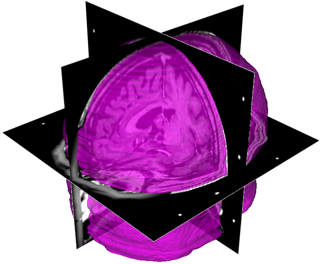
The 3D reconstruction of the predicted skull as displayed by 3DSlicer.
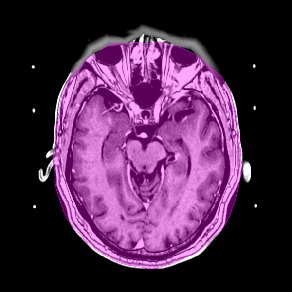
Overlay of the predicted skull segmentation on the T1-weighted image viewed on the axial plane.
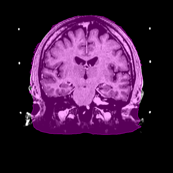
Overlay of the predicted skull segmentation on the T1-weighted image viewed on the coronal plane.
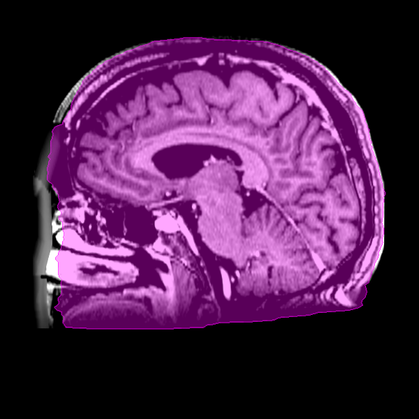
Overlay of the predicted skull segmentation on the T1-weighted image viewed on the sagittal plane.